One of the most important theoretical results in linear programming is that every LP has a corresponding dual program. Where, exactly, this dual comes from can often seem mysterious. Several years ago I answered a question on a couple of Stack Exchange sites giving an intuitive explanation for where the dual comes from. Those posts seem to have been appreciated, so I thought I would reproduce my answer here.
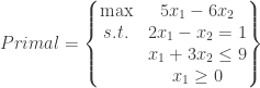
Suppose we have a primal problem as follows.
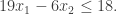
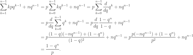
Now, suppose we want to use the primal’s constraints as a way to find an upper bound on the optimal value of the primal. If we multiply the first constraint by 9, the second constraint by 1, and add them together, we get  for the left-hand side and
  for the right-hand side. Since the first constraint is an equality and the second is an inequality, this implies
But since  , it’s also true that
  , and so

Therefore, 18 is an upper-bound on the optimal value of the primal problem.
Surely we can do better than that, though. Instead of just guessing 9 and 1 as the multipliers, let’s let them be variables. Thus we’re looking for multipliers  and
and  to force

Now, in order for this pair of inequalities to hold, what has to be true about and ? Let’s take the two inequalities one at a time.
The first inequality: 
We have to track the coefficients of the  and
and  variables separately. First, we need the total coefficient on the right-hand side to be at least 5. Getting exactly 5 would be great, but since , anything larger than 5 would also satisfy the inequality for . Mathematically speaking, this means that we need
  .
.
On the other hand, to ensure the inequality for the variable we need the total coefficient on the right-hand side to be exactly  . Since could be positive, we can’t go lower than , and since could be negative, we can’t go higher than (as the negative value for would flip the direction of the inequality). So for the first inequality to work for the variable, we’ve got to have
  .
.
The second inequality: 
Here we have to track the and variables separately. The variable comes from the first constraint, which is an equality constraint. It doesn’t matter if is positive or negative, the equality constraint still holds. Thus is unrestricted in sign. However, the variable comes from the second constraint, which is a less-than-or-equal to constraint. If we were to multiply the second constraint by a negative number that would flip its direction and change it to a greater-than-or-equal constraint. To keep with our goal of upper-bounding the primal objective, we can’t let that happen. So the variable can’t be negative. Thus we must have  .
.
Finally, we want to make the right-hand side of the second inequality as small as possible, as we want the tightest upper-bound possible on the primal objective. So we want to minimize  .
.
Putting all of these restrictions on and together we find that the problem of using the primal’s constraints to find the best upper bound on the optimal primal objective entails solving the following linear program:
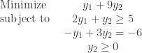
And that’s the dual.
It’s probably worth summarizing the implications of this argument for all possible forms of the primal and dual. The following table is taken from p. 214 of Introduction to Operations Research, 8th edition, by Hillier and Lieberman. They refer to this as the SOB method, where SOB stands for Sensible, Odd, or Bizarre, depending on how likely one would find that particular constraint or variable restriction in a maximization or minimization problem.
             Primal Problem                           Dual Problem
             (or Dual Problem)                        (or Primal Problem)

             Maximization                             Minimization

Sensible     <= constraint            paired with     nonnegative variable
Odd          =  constraint            paired with     unconstrained variable
Bizarre      >= constraint            paired with     nonpositive variable

Sensible     nonnegative variable     paired with     >= constraint
Odd          unconstrained variable   paired with     = constraint
Bizarre      nonpositive variable     paired with     <= constraint


 .
.  denote that claim that
  is true for some k; that is, suppose
  . Now,
  is the claim that
  . If
. If  , which proves that the truth of
  , all people in a group of size n share the same birthday.
 is true, as all people in a group of size 1 have the same birthday. Now, suppose that
  people. Single out one of those people; perhaps his name is Al. Without Al, we have a group of k people, all of whom must, by our inductive hypothesis, share the same birthday. Now, swap Al with one of those other k people. Now Al is in a group of k people. Again, by hypothesis all of them must share the same birthday. So Al must have the same birthday as all the others in his group. Thus these
  , and we remove Al from the group of two people, we then have Al and a group of size 1. Swapping Al with that one other person does put Al in a group of size 1, and he does share the same birthday as everyone else in the group (namely, just himself), but he doesn’t necessarily share the same birthday with that one other person. So
  , even though
  , together with combinatorial proofs of two formulas for this power sum. (An earlier version of some of the results in this paper actually appeared in a
 ![f: [m+1] \mapsto [n+1]](https://s0.wp.com/latex.php?latex=f%3A+%5Bm%2B1%5D+%5Cmapsto+%5Bn%2B1%5D&bg=ffffff&fg=333333&s=0&c=20201002) such that, for all
such that, for all ![i \in [m]](https://s0.wp.com/latex.php?latex=i+%5Cin+%5Bm%5D&bg=ffffff&fg=333333&s=0&c=20201002) ,
,  .
. this doesn’t work. The power sum as I stated it entails adding up n copies of 1 and so evaluates to n. On the other hand, the set
 ![[m]](https://s0.wp.com/latex.php?latex=%5Bm%5D&bg=ffffff&fg=333333&s=0&c=20201002) is the set
is the set  . This means that all
  functions from
 ![[1]](https://s0.wp.com/latex.php?latex=%5B1%5D&bg=ffffff&fg=333333&s=0&c=20201002) to
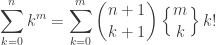
to ![[n+1]](https://s0.wp.com/latex.php?latex=%5Bn%2B1%5D&bg=ffffff&fg=333333&s=0&c=20201002) vacuously satisfy the condition in the theorem. The theorem as stated in the paper is off by 1, then, for the case
vacuously satisfy the condition in the theorem. The theorem as stated in the paper is off by 1, then, for the case  , so that we have the following.
 is the number of functions
  (and I am a fan of this convention in a combinatorial setting), this allows the formula to hold in the case
 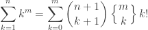 , and
, and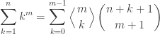 .
. , and
, and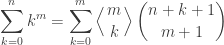 .
. . The definition for

 can be expressed as
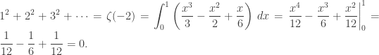
 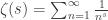 , for complex numbers s whose real part is greater than 1. By analytic continuation,
  .
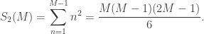
.  is given by
 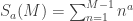 . (Sometimes M is given as the upper bound, but for this post it’s more convenient to use
  .)
.) and the power sum
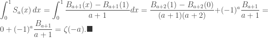
  . It’s due to Mináč [1], and I reproduce his proof here.
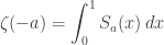 .
. from 0 to 1? Well, it’s also known that
  in M. For example,
 .
. .
. .
. ) are 0.
 .
.

 .
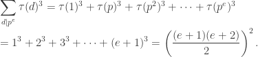
. , the function that counts the number of divisors of an integer:
 .
. , where p is prime. Since the only divisors of
  , the number of divisors of
  .
. . We have
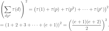
 and
and 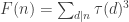 . What we’ve shown thus far is that
  .
.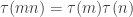 when m and n are relatively prime. This is one of the first properties you learn about
  is multiplicative.
  is also multiplicative. This is a special case of the more general result that the
  , take h to be the identity function; i.e.,
  .) This means that our functions f and F defined in the previous paragraph are both multiplicative.
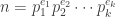 , we have
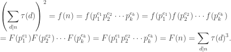

 are called
  has no integer solutions, using (with one exception) nothing more complicated than congruences.
 ,
,  . Looking at the equation modulo 8, then, we have
 .
. and reduce them modulo 8 we have
  . So there is no integer y that when squared is congruent to 7 modulo 8. Therefore, there is no solution to
  or
or  .
. . However, if we square the residues
  and reduce them modulo 4 we get
  . So there is no integer y that when squared is congruent to 2 modulo 4. Thus there is no solution to
  when
when  .
. . If
. If  has prime factors that are all equivalent to 1 modulo 4, then their product (i.e.,
  ) would be equivalent to 1 modulo 4. Thus
  , then
  . This means that
  . However, thanks to
  can have a solution to
  ,
, 